Outbreak Detection in Networks

Introduction

The general goal of outbreak detection in networks is that given a dynamic process spreading over a network, we want to select a set of nodes to detect the process efficiently. Outbreak detection in networks has many applications in real life. For example, where should we place sensors to quickly detect contaminations in a water distribution network? Which person should we follow on Twitter to avoid missing important stories?

The following figure shows the different effects of placing sensors at two different locations in a network:

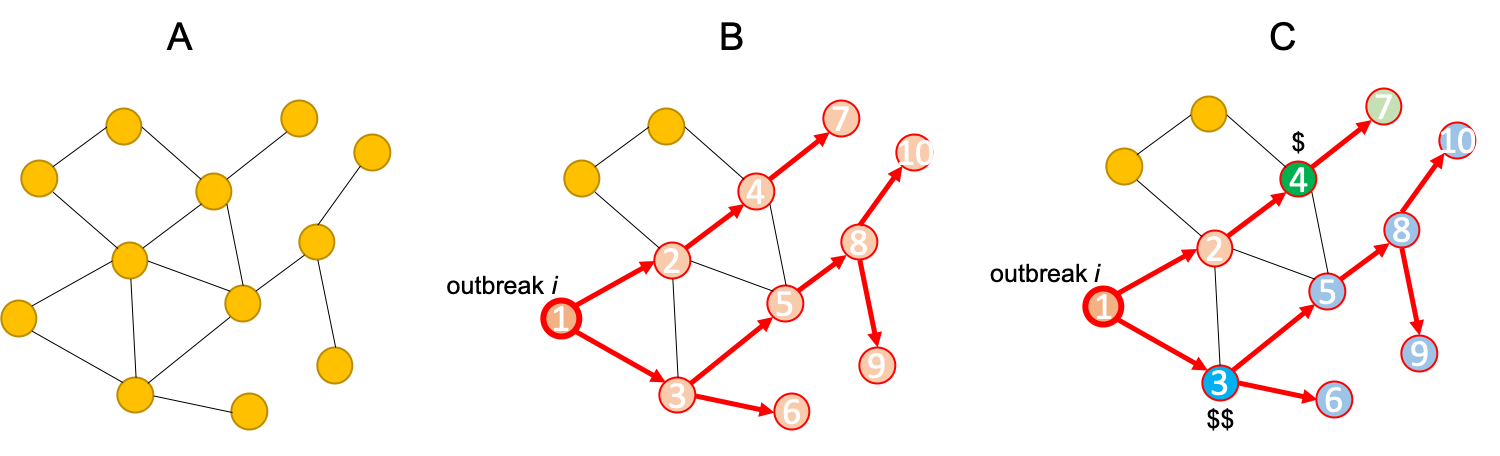(A) The given network. (B) An outbreak $i$ starts and spreads as shown. (C) Placing a sensor at the blue position saves more people and also detects earlier than placing a sensor at the green position, though costs more.

Problem Setup

The outbreak detection problem is defined as below:

• Given: a graph $G(V,E)$ and data on how outbreaks spread over this $G$ (for each outbreak $i$, we knew the time $T(u,i)$ when the outbreak $i$ contaminates node $u$).
• Goal: select a subset of nodes $S$ that maximize the expected reward:

where

• $p(i)$: probability of outbreak $i$ occurring
• $f_{i}(S)$: rewarding for detecting outbreak $i$ using “sensors” $S$It is obvious that $p(i)\cdot f_{i}(S)$ is the expected reward for detecting the outbreak $i$
• $B$: total budget of placing “sensors”

The Reward can be one of the following three:

• Minimize the time to detection
• Maximize the number of detected propagations
• Minimize the number of infected people

The Cost is context-dependent. Examples are:

• Reading big blogs is more time consuming
• Placing a sensor in a remote location is more expensive

Outbreak Detection Formalization

Objective Function for Sensor Placements

Define the penalty $\pi_{i}(t)$ for detecting outbreak $i$ at time $t$, which can be one of the following:Notice: in all the three cases detecting sooner does not hurt! Formally, this means, for all three cases, $\pi_{i}(t)$ is monotonically nondecreasing in $t$.

• Time to Detection (DT)
  • How long does it take to detect an outbreak?
  • Penalty for detecting at time $t$: $\pi_{i}(t)=t$
• Detection Likelihood (DL)
  • How many outbreaks do we detect?
  • Penalty for detecting at time $t$: $\pi_{i}(0)=0$, $\pi_{i}(\infty)=1$this is a binary outcome: $\pi_{i}(0)=0$ means we detect the outbreak and we pay 0 penalty, while $\pi_{i}(\infty)=1$ means we fail to detect the outbreak and we pay 1 penalty. That is we do not incur any penalty if we detect the outbreak in finite time, otherwise we incur penalty 1.
• Population Affected (PA)
  • How many people/nodes get infected during an outbreak?
  • Penalty for detecting at time $t$: $\pi_{i}(t)=$ number of infected nodes in the outbreak $i$ by time $t$

The objective reward function $f_{i}(S)$ of a sensor placement $S$ is defined as penalty reduction:

where $T(S,i)$ is the time when the set of “sensors” $S$ detects the outbreak $i$.

Claim 1: $f(S)=\sum_{i}p(i)\cdot f_{i}(S)$ is monotoneFor the definition of monotone, see Influence Maximization

Firstly, we do not reduce the penalty, if we do not place any sensors. Therefore, $f_{i}(\emptyset)=0$ and $f(\emptyset)=\sum_{i}p(i)\cdot f_{i}(\emptyset)=0$.

Secondly, for all $A\subseteq B\subseteq V$ ($V$ is all the nodes in $G$), $T(A,i)\geq T(B,i)$, and

Because $\pi_{i}(t)$ is monotonically nondecreasing in $t$ (see sidenote 2), $f_{i}(A)-f_{i}(B)<0$. Therefore, $f_{i}(S)$ is nondecreasing. It is obvious that $f(S)=\sum_{i}p(i)\cdot f_{i}(S)$ is also nondecreasing, since $p(i)\geq 0$.

Hence, $f(S)=\sum_{i}p(i)\cdot f_{i}(S)$ is monotone.

Claim 2: $f(S)=\sum_{i}p(i)\cdot f_{i}(S)$ is submodularFor the definition of submodular, see Influence Maximization

This is to proof for all $A\subseteq B\subseteq V$ $x\in V \setminus B$:

There are three cases when sensor $x$ detects the outbreak $i$:

1. $T(B,i)\leq T(A, i)<T(x,i)$ ($x$ detects late): nobody benefits. That is $f_{i}(A\cup\{x\})=f_{i}(A)$ and $f_{i}(B\cup\{x\})=f_{i}(B)$. Therefore, $f(A\cup \{x\})-f(A)=0= f(B\cup\{x\})-f(B)$
2. $T(B, i)\leq T(x, i)<T(A,i)$ ($x$ detects after $B$ but before $A$): $x$ only helps to improve the solution of $A$ but not $B$. Therefore, $f(A\cup \{x\})-f(A)\geq 0 = f(B\cup\{x\})-f(B)$
3. $T(x, i)<T(B,i)\leq T(A,i)$ ($x$ detects early): $f(A\cup \{x\})-f(A)=[\pi_{i}(\infty)-\pi_{i}(T(x,t))]-f_{i}(A)$$\geq [\pi_{i}(\infty)-\pi_{i}(T(x,t))]-f_{i}(B) = f(B\cup\{x\})-f(B)$Inequality is due to the nondecreasingness of $f_{i}(\cdot)$, i.e. $f_{i}(A)\leq f_{i}(B)$ (see Claim 1).

Therefore, $f_{i}(S)$ is submodular. Because $p(i)\geq 0$, $f(S)=\sum_{i}p(i)\cdot f_{i}(S)$ is also submodular.Fact: a non-negative linear combination of submodular functions is a submodular function.

We know that the Hill Climbing algorithm works for optimizing problems with nondecreasing submodular objectives. However, it does not work well in this problem:

• Hill Climbing only works for the cases that each sensor costs the same. For this problem, each sensor has cost $c(s)$.
• Hill Climbing is also slow: at each iteration, we need to re-evaluate marginal gains of all nodes. The run time is $O(\mid V\mid\cdot k)$ for placing $k$ sensors.

Hence, we need a new fast algorithm that can handle cost constraints.

CELF: Algorithm for Optimziating Submodular Functions Under Cost Constraints

Bad Algorithm 1: Hill Climbing that ignores the cost

Algorithm

• Ignore sensor cost $c(s)$
• Repeatedly select sensor with highest marginal gain
• Do this until the budget is exhausted

This can fail arbitrarily bad! Example:

• Given $n$ sensors and a budget $B$
• $s_{1}$: reward $r$, cost $B$
• $s_{2}$,…, $s_{n}$: reward $r-\epsilon$, cost $\epsilon$ ($\epsilon$ is an arbitrary positive small number)
• Hill Climbing always prefers $s_{1}$ to other cheaper sensors, resulting in an arbitrarily bad solution with reward $r$ instead of the optimal solution with reward $\frac{B(r-\epsilon)}{\epsilon}$, when $\epsilon \rightarrow 0$.

Bad Algorithm 2: optimization using benefit-cost ratio

Algorithm

• Greedily pick the sensor $s_{i}$ that maximizes the benefit to cost ratio until the budget runs out, i.e. always pick

This can fail arbitrarily bad! Example:

• Given 2 sensors and a budget $B$
• $s_{1}$: reward $2\epsilon$, cost $\epsilon$
• $s_{2}$: reward $B$, cost $B$
• Then the benefit ratios for the first selection are: 2 and 1, respectively
• This algorithm will pick $s_{1}$ and then cannot afford $s_{2}$, resulting in an arbitrarily bad solution with reward $2\epsilon$ instead of the optimal solution $B$, when $\epsilon \rightarrow 0$.

Solution: CELF (Cost-Effective Lazy Forward-selection)

CELF is a two-pass greedy algorithm [Leskovec et al. 2007]:

• Get solution $S'$ using unit-cost greedy (Bad Algorithm 1)
• Get solution $S''$ using benefit-cost greedy (Bad Algorithm 2)
• Final solution $S=\arg\max[f(S'), f(S'')]$

Approximation Guarantee

• CELF achieves $\frac{1}{2}(1-\frac{1}{e})$ factor approximation.

CELF also uses a lazy evaluation of $f(S)$ (see below) to speedup Hill Climbing.

Lazy Hill Climbing: Speedup Hill Climbing

Intuition

• In Hill Climbing, in round $i+1$, we have picked $S_{i}=\{S_{1},...,S_{i}\}$ sensors. Now, pick $s_{i+1}=\arg\max_{u}f(S_{i}\cup \{u\})-f(S_{i})$
• By submodularity $f(S_{i}\cup\{u\})-f(S_{i})\geq f(S_{j}\cup\{u\})-f(S_{j})$ for $i<j$.
• Let $\delta_{i}(u)=f(S_{i}\cup\{u\})-f(S_{i})$ and $\delta_{j}(u)=f(S_{j}\cup\{u\})-f(S_{j})$ be the marginal gains. Then, we can use $\delta_{i}$ as upper bound on $\delta_{j}$ for ($j>i$)

Lazy Hill Climbing Algorithm:

• Keep an ordered list of marginal benefits $\delta_{i-1}$ from previous iteration
• Re-evaluate $\delta_{i}$ only for the top nodes
• Reorder and prune from the top nodes

The following figure show the process.

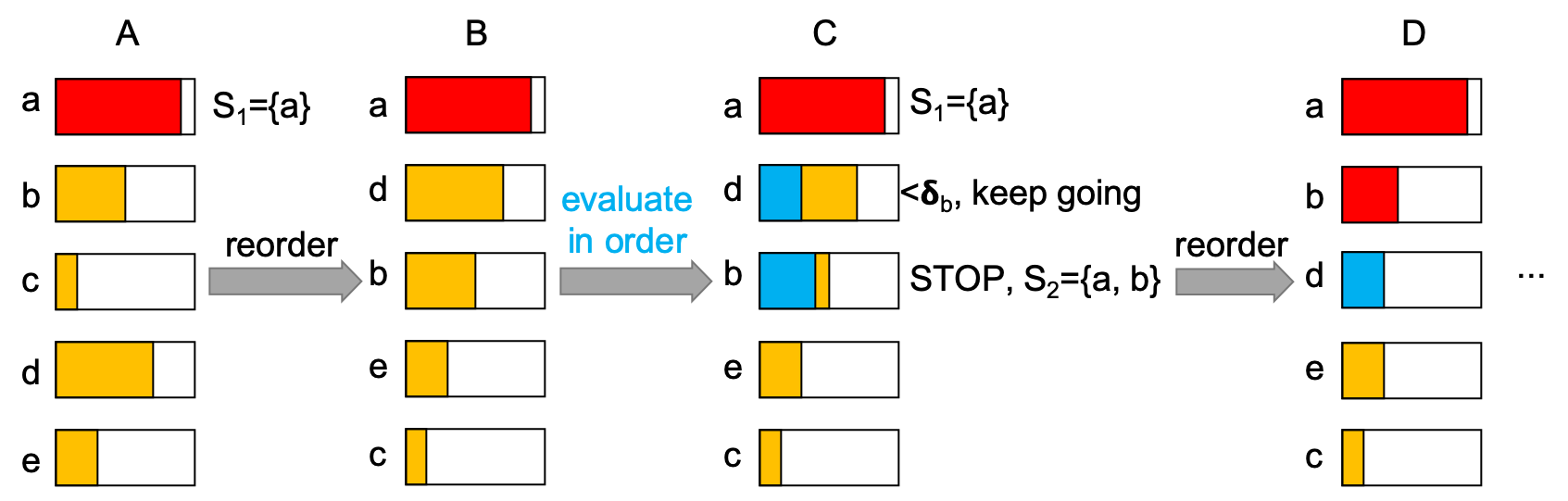
(A) Evaluate and pick the node with the largest marginal gain $\delta$. (B) reorder the marginal gain for each sensor in decreasing order. (C) Re-evaluate the $\delta$s in order and pick the possible best one by using previous $\delta$s as upper bounds. (D) Reorder and repeat.

Note: the worst case of Lazy Hill Climbing has the same time complexity as normal Hill Climbing. However, it is on average much faster in practice.

Data-Dependent Bound on the Solution Quality

Introduction

• Value of the bound depends on the input data
• On “easy data”, Hill Climbing may do better than the $(1-\frac{1}{e})$ bound for submodular functions

Data-Dependent Bound

Suppose $S$ is some solution to $f(S)$ subjected to $\mid S \mid\leq k$, and $f(S)$ is monotone and submodular.

• Let $OPT={t_{i},...,t_{k}}$ be the optimal solution
• For each $u$ let $\delta(u)=f(S\cup\{u\})-f(S)$
• Order $\delta(u)$ so that $\delta(1)\geq \delta(2)\geq...$
• Then, the data-dependent bound is $f(OPT)\leq f(S)+\sum^{k}_{i=1}\delta(i)$

Proof:For the first inequality, see the lemma in 3.4.1 of this handout. For the last inequality in the proof: instead of taking $t_{i}\in OPT$ of benefit $\delta(t_{i})$, we take the best possible element $\delta(i)$, because we do not know $t_{i}$.

Note:

• This bound hold for the solution $S$ (subjected to $\mid S \mid\leq k$) of any algorithm having the objective function $f(S)$ monotone and submodular.
• The bound is data-dependent, and for some inputs it can be very “loose” (worse than $(1-\frac{1}{e})$)