Influence Maximization

Motivation

Identification of influential nodes in a network has important practical uses. A good example is “viral marketing”, a strategy that uses existing social networks to spread and promote a product. A well-engineered viral marking compaign will identify the most influential customers, convince them to adopt and endorse the product, and then spread the product in the social network like a virus.

The key question is how to find the most influential set of nodes? To answer this question, we will first look at two classical cascade models:

• Linear Threshold Model
• Independent Cascade Model

Then, we will develop a method to find the most influential node set in the Independent Cascade Model.

Linear Threshold Model

In the Linear Threshold Model, we have the following setup:

• A node $v$ has a random threshold $\theta_{v} \sim U[0,1]$
• A node $v$ influenced by each neighbor $w$ according to a weight $b_{v,w}$, such that

• A node $v$ becomes active when at least $\theta_{v}$ fraction of its neighbors are active. That is

The following figure demonstrates the process:

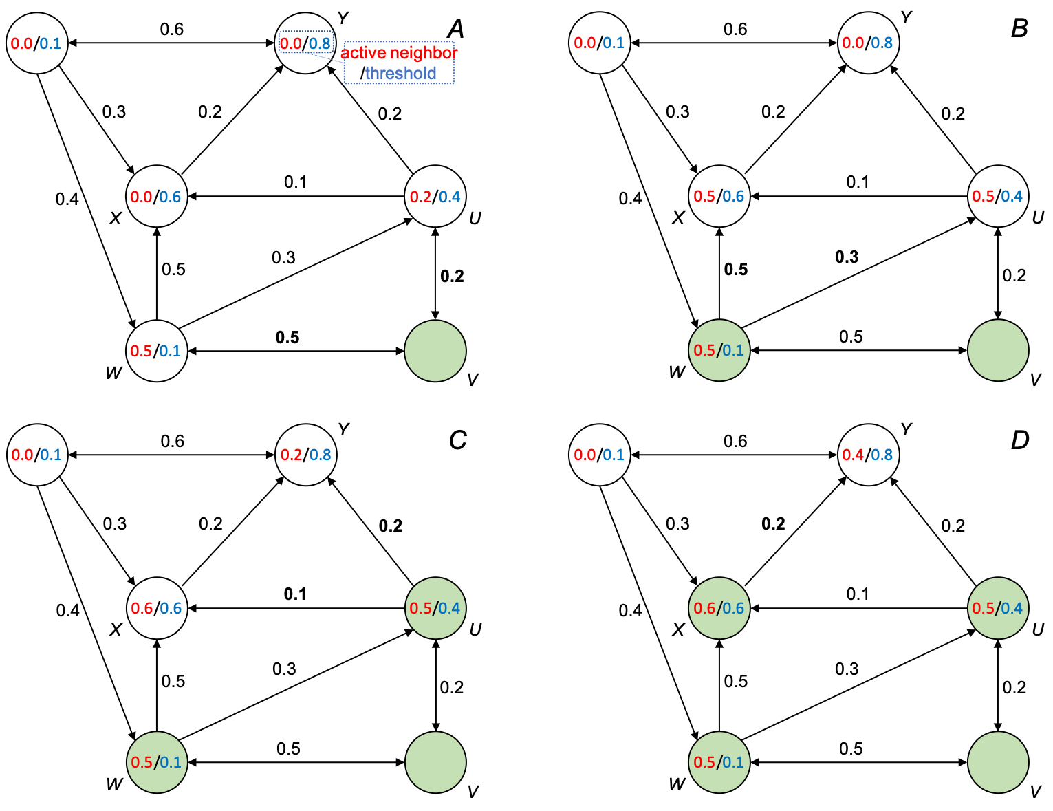
(A) node V is activated and influences W and U by 0.5 and 0.2, respectively; (B) W becomes activated and influences X and U by 0.5 and 0.3, respectively; (C) U becomes activated and influences X and Y by 0.1 and 0.2, respectively; (D) X becomes activated and influences Y by 0.2; no more nodes can be activated; process stops.

Independent Cascade Model

In this model, we model the influences (activation) of nodes based on probabilities in a directed graph:

• Given a directed finite graph $G=(V, E)$
• Given a node set $S$ starts with a new behavior (e.g. adopted new product and we say they are active)
• Each edge $(v, w)$ has a probability $p_{vw}$
• If node $v$ becomes active, it gets one chance to make $w$ active with probability $p_{vw}$
• Activation spread through the network

Note:

• Each edge fires only once
• If $u$ and $v$ are both active and link to $w$, it does not matter which tries to activate $w$ first

Influential Maximization (of the Independent Cascade Model)

Definitions

• Most influential Set of size $k$ ($k$ is a user-defined parameter) is a set $S$ containing $k$ nodes that if activated, produces the largest expectedWhy “expected cascade size”? Due to the stochastic nature of the Independent Cascade Model, node activation is a random process, and therefore, $f(S)$ is a random variable. In practice, we would like to compute many random simulations and then obtain the expected value $f(S)=\frac{1}{\mid I\mid}\sum_{i\in I}f_{i}(S)$, where $I$ is a set of simulations. cascade size $f(S)$.
• Influence set $X_{u}$ of node $u$ is the set of nodes that will be eventually activated by node $u$. An example is shown below.

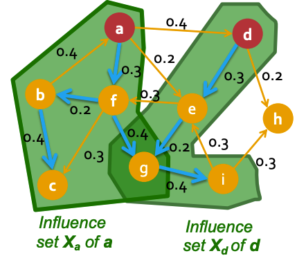
Red-colored nodes a and b are active. The two green areas enclose the nodes activated by a and b respectively, i.e. $X_{a}$ and $X_{b}$.

Note:

• It is clear that $f(S)$ is the size of the union of $X_{u}$: $f(S)=\mid\cup_{u\in S}X_{u}\mid$.
• Set $S$ is more influential, if $f(S)$ is larger

Problem Setup

The influential maximization problem is then an optimization problem:

This problem is NP-hard [Kempe et al. 2003]. However, there is a greedy approximation algorithm–Hill Climbing that gives a solution $S$ with the following approximation guarantee:

where $OPT$ is the globally optimal solution.

Hill Climbing

Algorithm: at each step $i$, activate and pick the node $u$ that has the largest marginal gain $\max_{u}f(S_{i-1}\cup\{u\})$:

• Start with $S_{0}=\{\}$
• For $i=1...k$
  • Activate node $u\in V\setminus S_{i-1}$ that $\max_{u}f(S_{i-1}\cup\{u\})$
  • Let $S_{i}=S_{i-1}\cup\{u\}$

Claim: Hill Climbing produces a solution that has the approximation guarantee $f(S)\geq(1-\frac{1}{e})f(OPT)$.

Proof of the Approximation Guarantee of Hill Climbing

Definition of Monotone: if $f(\emptyset)=0$ and $f(S)\leq f(T)$ for all $S\subseteq T$, then $f(\cdot)$ is monotone.

Definition of Submodular: if $f(S\cup \{u\})-f(S)\geq f(T\cup\{u\})-f(T)$ for any node $u$ and any $S\subseteq T$, then $f(\cdot)$ is submodular.

Theorem [Nemhauser et al. 1978]:also see this handout if $f(\cdot)$ is monotone and submodular, then the $S$ obtained by greedily adding $k$ elements that maximize marginal gains satisfies

Given this theorem, we need to prove that the largest expected cascade size function $f(\cdot)$ is monotone and submodular.

It is clear that the function $f(\cdot)$ is monotone based on the definition of $f(\cdot)$If no nodes are active, then the influence is 0. That is $f(\emptyset)=0$. Because activating more nodes will never hurt the influence, $f(U)\leq f(V)$ if $U\subseteq V$., and we only need to prove $f(\cdot)$ is submodular.

Fact 1 of Submodular Functions: $f(S)=\mid \cup_{k\in S}X_{k}\mid$ is submodular, where $X_{k}$ is a set. Intuitively, the more sets you already have, the less new “area”, a newly added set $X_{k}$ will provide.

Fact 2 of Submodular Functions: if $f_{i}(\cdot)$ are submodular and $c_{i}\geq0$, then $F(\cdot)=\sum_{i}c_{i} f_{i}(\cdot)$ is also submodular. That is a non-negative linear combination of submodular functions is a submodular function.

Proof that $f(\cdot)$ is Submodular: we run many simulations on graph G (see sidenote 1). For the simulated world $i$, the node $v$ has an activation set $X^{i}_{v}$, then $f_{i}(S)=\mid\cup_{v\in S}X^{i}_{v}\mid$ is the size of the cascades of $S$ for world $i$. Based on Fact 1, $f_{i}(S)$ is submodular. The expected influence set size $f(S)=\frac{1}{\mid I\mid}\sum_{i\in I}f_{i}(S)$ is also submodular, due to Fact 2. QED.

Evaluation of $f(S)$ and Approximation Guarantee of Hill Climbing In Practice: how to evaluate $f(S)$ is still an open question. The estimation achieved by simulating a number of possible worlds is a good enough evaluation [Kempe et al. 2003]:

• Estimate $f(S)$ by repeatedly simulating $\Omega(n^{\frac{1}{\epsilon}})$ possible worlds, where $n$ is the number of nodes and $\epsilon$ is a small positive real number
• It achieves $(1\pm \epsilon)$-approximation to $f(S)$
• Hill Climbing is now a $(1-\frac{1}{e}-\epsilon)$-approximation

Speed-up Hill Climbing by Sketch-Based Algorithms

Time complexity of Hill Climbing

To find the node $u$ that $\max_{u}f(S_{i-1}\cup\{u\})$ (see the algorithm above):

• we need to evaluate the $X_{u}$ (the influence set) of each of the remaining nodes which has the size of $O(n)$ ($n$ is the number of nodes in $G$)
• for each evaluation, it takes $O(m)$ time to flip coins for all the edges involved ($m$ is the number of edges in $G$)
• we also need $R$ simulations to estimate the influence set ($R$ is the number of simulations/possible worlds)

We will do this $k$ (number of nodes to be selected) times. Therefore, the time complexity of Hill Climbing is $O(k\cdot n \cdot m \cdot R)$, which is slow. We can use sketches [Cohen et al. 2014] to speed up the evaluation of $X_{u}$ by reducing the evaluation time from $O(m)$ to $O(1)$Besides sketches, there are other proposed approaches for efficiently evaluating the influence function: approximation by hypergraphs [Borgs et al. 2012], approximating Riemann sum [Lucier et al. 2015], sparsification of influence networks [Mathioudakis et al. 2011], and heuristics, such as degree discount [Chen et al. 2009]..

Single Reachability Sketches

• Take a possible world $G^{i}$ (i.e. one simulation of the graph $G$ using the Independent Cascade Model)
• Give each node a uniform random number $\in [0,1]$
• Compute the rank of each node $v$, which is the minimum number among the nodes that $v$ can reach in this world.

Intuition: if $v$ can reach a large number of nodes, then its rank is likely to be small. Hence, the rank of node $v$ can be used to estimate the influence of node $v$ in $G^{i}$.

However, influence estimation based on Single Reachability Sketches (i.e. single simulation of $G$ ) is inaccurate. To make a more accurate estimate, we need to build sketches based on many simulationsThis is similar to take an average of $f_{i}(S)$ in sidenote 1, but in this case, it is achieved by using Combined Reachability Sketches., which leads to the Combined Reachability Sketches.

Combined Reachability Sketches

In Combined Reachability Sketches, we simulate several possible worlds and keep the smallest $c$ values among the nodes that $u$ can reach in all the possible worlds.

• Construct Combined Reachability Sketches:

  • Generate a number of possible worlds
  • For node $u$, assign uniformly distributed random numbers $r^{i}_{v}\in[0,1]$ to all $(v, i)$ pairs, where $v$ is the node in $u$’s reachable nodes set in the world $i$.
  • Take the $c$ smallest $r^{i}_{v}$ as the Combined Reachability Sketches

• Run Greedy for Influence Maximization:

  • Whenever the greedy algorithm asks for the node with the largest influence, pick node $u$ that has the smallest value in its sketch.
  • After $u$ is chosen, find its influence set $X^{i}_{u}$, mark the $(v, i)$ as infected and remove their $r^{i}_{v}$ from the sketches of other nodes.

Note: using Combined Reachability Sketches does not provide an approximation guarantee on the true expected influence but an approximation guarantee with respect to the possible worlds considered.