Measuring Networks and Random Graphs
Measuring Networks via Network Properties
In this section, we study four key network properties to characterize a graph: degree distribution, path length, clustering coefficient, and connected components. Definitions will be presented for undirected graphs, but can be easily extended to directed graphs.
Degree Distribution
The degree distribution measures the probability that a randomly chosen node has degree . The degree distribution of a graph can be summarized by a normalized histogram, where we normalize the histogram by the total number of nodes.
We can compute the degree distribution of a graph by . Here, is the number of nodes with degree and is the number of nodes. One can think of degree distribution as the probability that a randomly chosen node has degree .
To extend these definitions to a directed graph, compute separately both in-degree and out-degre distribution.
Paths in a Graph
A path is a sequence of nodes in which each node is linked to the next one:
such that
The distance (shortest path, geodesic) between a pair of nodes is defined as the number of edges along the shortest path connecting the nodes. If two nodes are not connected, the distance is usually defined as infinite (or zero). One can also think of distance as the smallest number of nodes needed to traverse to get form one node to another.
In a directed graph, paths need to follow the direction of the arrows. Thus, distance is not symmetric for directed graphs. For a graph with weighted edges, the distance is the minimum number of edge weight needed to traverse to get from one node to another.
The average path length of a graph is the average shortest path between all connected nodes. We compute the average path length as
where is the max number of edges or node pairs; that is, and is the distance from node to node . Note that we only compute the average path length over connected pairs of nodes, and thus ignore infinite length paths.
Clustering Coefficient
The clustering coefficient (for undirected graphs) measures what proportion of node ’s neighbors are connected. For node with degree , we compute the clustering coefficient as
where is the number of edges between the neighbors of node . Note that . Also, the clustering coefficient is undefined for nodes with degree 0 or 1.
We can also compute the average clustering coefficent as
The average clustering coefficient allows us to see if edges appear more densely in parts of the network. In social networks, the average clustering coefficient tends to be very high indicating that, as we expect, friends of friends tend to know each other.
Connectivity
The connectivity of a graph measures the size of the largest connected component. The largest connected component is the largest set where any two vertices can be joined by a path.
To find connected components:
- Start from a random node and perform breadth first search (BFS)
- Label the nodes that BFS visits
- If all the nodes are visited, the netowrk is connected
- Otherwise find an unvisited node and repeat BFS
The Erdös-Rényi Random Graph Model
The Erdös-Rényi Random Graph Model is the simplest model of graphs. This simple model has proven networks properties and is a good baseline to compare real-world graph properties with.
This random graph model comes in two variants:
- : undirected graph on nodes where each edge appears IID with probability
- : undirected graph with nodes, and edges picked uniformly at random
Note that both the and graph are not uniquely determined, but rather the result of a random procedure. Generating each graph multiple times results in different graphs.
Some Network Properties of
The degree distribution of is binomial. Let denotes the fraction of nodes with degree , then
The mean and variance of a binomial distribution respectively are and . Below we include an image of binomial distributions for different paramters. Note that a binomial distribution is a discrete analogue of a Gaussian and has a bell-shape.
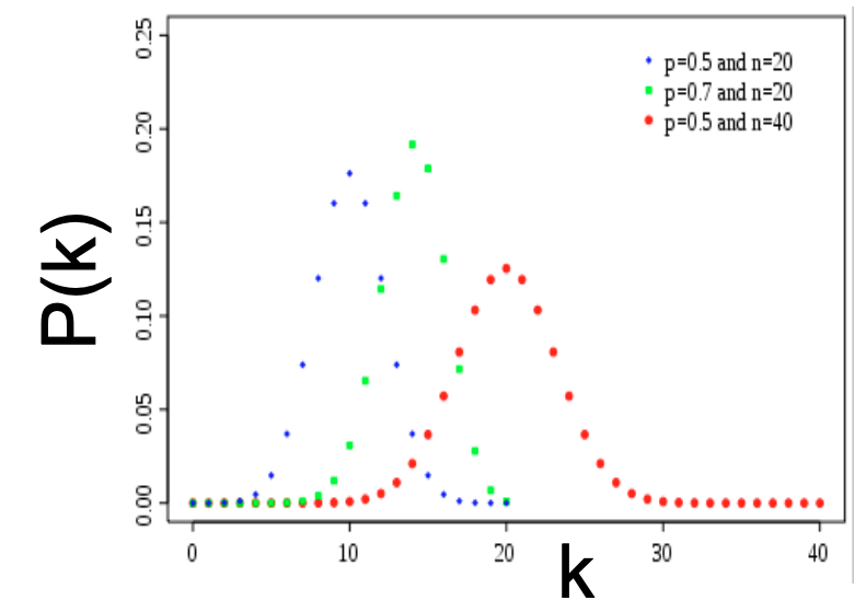
One property of binomial distributions is that by the law of numbers, as the network size increases, the distribution becomes increasingly narrow. Thus, we are increasingly confidence that the degree of a ndoe is in the vicinity of . If the graph has an infinite number of nodes, all nodes will have the same degree.
The Clustering Coefficient of
Recall that the clustering coefficient is computed as where is the number of edges between ’s neighbors. Edges in appear IID with probability , so the expected for is
This is because is the number of distinct pairs of neighbors of node of degree , and each pair is connected with probability .
Thus, the expected clustering coefficient is
where is the average degree. From this, we can see that the clustering coefficient of is very small. If we generate bigger and bigger graphs with fixed average degree , then decreases with graph size . as .
The Path Length of
To discuss the path length of , we fist introduce the concept of expansion. Graph has expansion if , the number of edges leaving . Expansion answers the question ‘‘if we pick a random set of nodes, how many edges are going to leave the set?’’ Expansion is a measure of robustness: to disconnect nodes, one must cut edges.
Equivalently, we can say a graph has an expansion such that
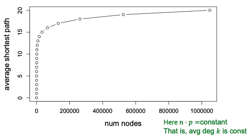
An important fact about expansion is that in a graph with nodes with expansion , for all pairs of nodes, there is a path of connecting them. For a random graph, , so . Thus, we can see that random graphs have good expansion so it takes as logarithmic number of steps for BFS to visit all nodes.
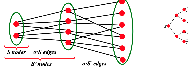
Thus, the path length of is . From this result, we can see that can grow very large, but nodes will still remain a few hops apart.
The Connectivity of
The graphic below shows the evolution of a random graph. We can see that there is an emergence of a giant component when average degree or . If , then all components are of size . If , there exists 1 component of size , and all other components have size . In other words, if , we expect a single large component. Additionally, in this case, each node has at least one edge in expectation.

Analyzing the Properties of
In grid networks, we achieve triadic closures and high clustering, but long average path length.
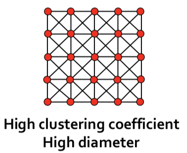
In random networks, we achieve short average path length, but low clustering.
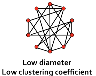
Given the two above graph structures, it may seem unintuitive that graphs can have short average path length while also having high clustering. However, most real-world networks have such properties as in the below table, where refers to the average shortest path length, refers to the average clustering coefficient, and random graphs were generated with the same average degree as actual networks for comparison.
| Network | ||||
|---|---|---|---|---|
| Film actors | 3.65 | 2.99 | 0.79 | 0.00027 |
| Power Grid | 18.70 | 12.40 | 0.080 | 0.005 |
| C. elegans | 2.65 | 2.25 | 0.28 | 0.05 |
Networks that meet the above criteria of both high clustering and small average path length (mathematically defined as where is average path length and is the total number of nodes in the network) are referred to as small world networks.
The Small World Random Graph Model
In 1998, Duncan J. Watts and Steven Strogatz came up with a model for constructing a family of networks with both high clustering and short average path length. They termed this model the ‘‘small world model’’. To create such a model, we employ the following steps:
-
Start with low-dimensional regular attic (ring) by connecting each node to neighbors on its right and neighbors on its left, with .
-
Rewire each edge with probability by moving its endpoint to a randomly chosen node.Several variants of rewiring exist. To learn more, see M. E. J. Newman. Networks, Second Edition, Oxford University Press, Oxford (2018)
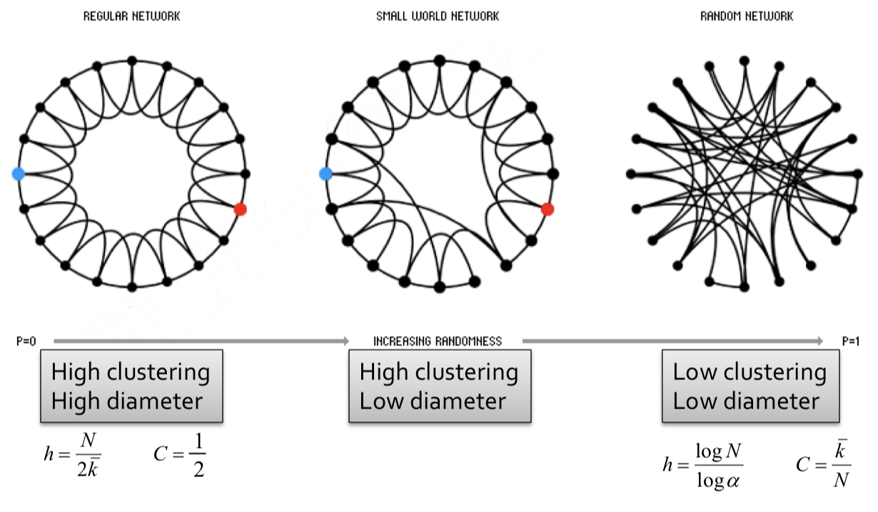
Then, we make the following observations:
- At where no rewiring has occured, this remains a grid network with high clustering, high diameter.
- For some edges have been rewired, but most of the structure remains. This implies both locality and shortcuts. This allows for both high clustering and low diameter.
- At where all edges have been randomly rewired, this is a Erdős–Rényi (ER) random graph with low clustering, low diameter.
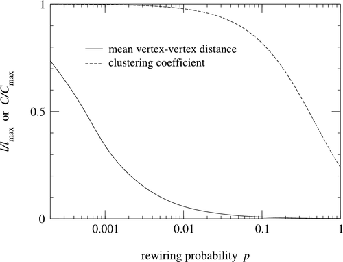
Small world models are parameterized by the probability of rewiring . By examining how the clustering coefficient and the average path length vary with values of , we see that average path length falls off much faster as increases, while the clustering coefficient remains relatively high. Rewiring introduces shortcuts, which allows for average path length to decrease even while the structure remains relatively strong (high clustering).
From a social network perspective, this phenomenon is intuitive. While most our friends are local, but we also have a few long distance friendships in different countries which is enough to collapse the diameter of the human social network, explaining the popular notion of “Six Degrees of Seperation”.
Two limitations of the Watts-Strogatz Small World Model are that its degree distribution does not match the power-law distributions of real world networks, and it cannot model network growth as the size of network is assumed.
The Kronecker Random Graph Model
Models of graph generation have been studied extensively. Such models allow us to generate graphs for simulations and hypothesis testing when collecting the real graph is difficult, and also forces us to examine the network properties that generative models should obey to be considered realistic.
In formulating graph generation models, there are two important considerations. First, the ability to generate realistic networks, and second, the mathematical tractability of the models, which allows for the rigorous analysis of network properties.
The Kronecker Graph Model is a recursive graph generation model that combines both mathematical tractability and realistic static and temporal network properties. The intuition underlying the Kronecker Graph Model is self-similarity, where the whole has the same shape as one or more of its parts.

The Kronecker product, a non-standard matrix operation, is a way to generate self-similar matrices.
The Kronecker Product
The Kronecker product is denoted by . For two arbitarily sized matrices and , such that
For example, we have that
To use the Kronecker product in graph generation, we define the Kronecker product of two graphs as the Kronecker product of the adjacency matrices of the two graphs.
Beginning with the initiator matrix (an adjacency matrix of a graph), we iterate the Kronecker product to produce successively larger graphs, , such that the Kronecker graph of order is defined by
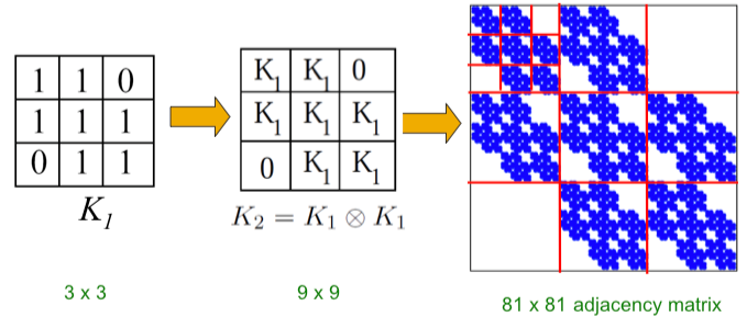
Intuitively, the Kronecker power construction can be imagined as recursive growth of the communities within the graph, with nodes in the community recursively getting expanded into miniature copies of the community.
The choice of the Kronecker initiator matrix can be varied, which iteratively affects the structure of the larger graph.
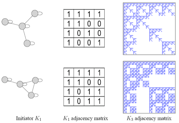
Stochastic Kronecker Graphs
Up to now, we have only considered initiator matrices with binary values . However, such graphs generated from such initiator matrices have “staircase” effects in the degree distributions and other properties: individual values occur very frequently because of the discrete nature of .
To negate this effect, stochasticity is introduced by relaxing the assumption that the entries in the initiator matrix can only take binary values. Instead entries in can take values on the interval , and each represents the probability of that particular edge appearing. Then the matrix (and all the generated larger matrix products) represent the probability distribution over all possible graphs from that matrix.
More concretely, for probaility matrix , we compute the Kronecker power as the large stochastic adjacency matrix. Each entry in then represents the probability of edge appearing.
Note that the probabilities do not have to sum up to 1 as each the probability of each edge appearing is independent from other edges.
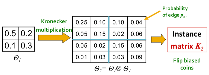
To obtain an instance of a graph, we then sample from the distribution by sampling each edge with probability given by the corresponding entry in the stochastic adjacency matrix. The sampling can be thought of as the outcomes of flipping biased coins where the bias is parameterized from each entry in the matrix.
However, this means that the time to naively generate an instance is quadratic in the size of the graph, ; with 1 million nodes, we perform 1 million x 1 million coin flips.
Fast Generation of Stochastic Kronecker Graphs
A fast heuristic procedure that takes time linear in the number of edges to generate a graph exists.
The general idea can be described as follows: for each edge, we recurively choose sub-regions of the large stochastic matrix with probability proportional to until we descend to a single cell of the large stochastic matrix. We place the edge there. For a Kronecker graph of power, , the descent will take steps.
For example, we consider the case where is a matrix, such that
For graph with nodes:
- Create normalized matrix
- For each edge:
- For :
- Start with
- Pick the row, column with probability
- Descend into quadrant based on step of
- Set
- Set
- Add edge to
- For :
If , and on each step , we pick quadrants respectively based on the normalized probabilities from , then
Hence, we add edge to the graph.
In practice, the stochastic Kronecker graph model is able to generate graphs that match the properties of real world networks well. To read more about the Kronecker Graph models, refer to J Leskovec et al., Kronecker Graphs: An Approach to Modeling Networks (2010).Estimating the initator matrice and fitting Kronecker Graphs to real world networks is also discussed in this work.
| Index | Previous | Next |