Node Representation Learning
In this section, we study several methods to represent a graph in the embedding space. By “embedding” we mean mapping each node in a network into a low-dimensional space, which will give us insight into nodes’ similarity and network structure. Given the widespread prevalence of graphs on the web and in the physical world, representation learning on graphs plays a significant role in a wide range of applications, such as link prediction and anomaly detection. However, modern machine learning algorithms are designed for simple sequence or grids (e.g., fixed-size images/grids, or text/sequences), networks often have complex topographical structures and multimodel features. We will explore embedding methods to get around the difficulties.
Embedding Nodes
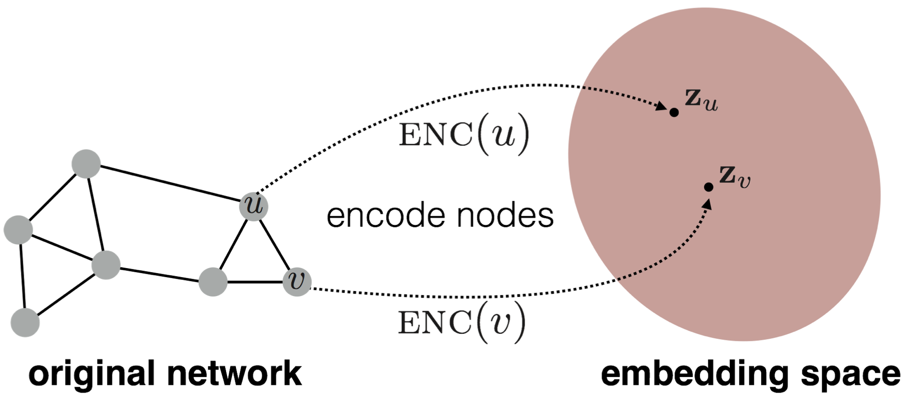
The goal of node embedding is to encode nodes so that similarity in the embedding space (e.g., dot product) approximates similarity in the original network, the node embedding algorithms we will explore generally consist of three basic stages:
-
Define an encoder (i.e., a mapping from nodes to embeddings). Below we include a diagram to illustrate the process, encoder maps node and to low-dimensional vector and :
- Define a node similarity function (i.e., a measure of similarity in the original network), it specifies how the relationships in vector space map to the relationships in the original network.
- Optimize the parameters of the encoder so that similarity of and in the network approximate the dot product between node embeddings: .
“Shallow” Encoding
How to define a encoder to map nodes into a embedding space?
“Shallow” encoding is the simplest encoding approach, it means encoder is just an embedding-lookup and it could be represented as:
Each column in matrix indicates a node embedding, the total number of rows in equals to the dimension/size of embeddings. is the indicator vector with all zeros except a one in column indicating node . We see that each node is assigned to a unique embedding vector in “shallow” encoding. There are many ways to generate node embeddings (e.g., DeepWalk, node2vec, TransE), key choices of methods depend on how they define node similarity.
Random Walk
Now let’s try to define node similarity. Here we introduce Random Walk, an efficient and expressive way to define node similarity Random walk has a flexible stochastic definition of node similarity that incorporates both local and higher-order neighborhood information, also it does not need to consider all node pairs when training; only need to consider pairs that co-occur on random walks. and train node embeddings: given a graph and a starting point, we select a neighbor of it at random, and move to this neighbor; then we select a neighbor of this point at random, and move to it, etc. The (random) sequence of points selected this way is a random walk on the graph. So is defined as the probability that and co-occur on a random walk over a network. We can generate random-walk embeddings following these steps:
- Estimate probability of visiting node on a random walk starting from node using some random walk strategy . The simplest idea is just to run fixed-length, unbiased random walks starting from each node (i.e., DeepWalk from Perozzi et al., 2013).
- Optimize embeddings to encode these random walk statistics, so the similarity between embeddings (e.g., dot product) encodes Random Walk similarity.
Random walk optimization and Negative Sampling
Since we want to find embedding of nodes to d-dimensions that preserve similarity, we need to learn node embedding such that nearby nodes are close together in the network. Specifically, we can define nearby nodes as neighborhood of node obtained by some strategy . Let’s recall what we learn from random walks, we could run short fixed-length random walks starting from each node on the graph using some strategy to collect , which is the multiset of nodes visited on random walks starting from . Note that can have repeat elements since nodes can be visited multiple times on random walks. Then we might optimize embeddings to maximize the likelihood of random walk co-occurrences, we compute loss function as:
where we parameterize using softmax:
Put it together:
To optimize random walk embeddings, we need to find embeddings that minimize . But doing this naively without any changes is too expensive, nested sum over nodes gives complexity. Here we introduce Negative Sampling To read more about negative sampling, refer to Goldberg et al., word2vec Explained: Deriving Mikolov et al.’s Negative-Sampling Word-Embedding Method (2014). to approximate the loss. Technically, Negative sampling is a different objective, but it is a form of Noise Contrastive Estimation (NCE) which approximately maximizes the log probability of softmax. New formulation corresponds to using a logistic regression (sigmoid func.) to distinguish the target node from nodes sampled from background distribution such that
means random distribution over all nodes. Instead of normalizing with respect to all nodes, we just normalize against random “negative samples” . In this way, we need to sample negative nodes proportional to degree to compute the loss function. Note that higher gives more robust estimates, but it also corresponds to higher bias on negative events. In practice, we choose between 5 to 20.
Node2vec
So far we have described how to optimize embeddings given random walk statistics, What strategies should we use to run these random walks? As we mentioned before, the simplest idea is to run fixed-length, unbiased random walks starting from each node (i.e., DeepWalk from Perozzi et al., 2013), the issue is that such notion of similarity is too constrained. We observe that flexible notion of network neighborhood of node leads to rich node embeddings, the idea of Node2Vec is using flexible, biased random walks that can trade off between local and global views of the network (Grover and Leskovec, 2016). Two classic strategies to define a neighborhood of a given node are BFS and DFS:
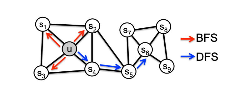
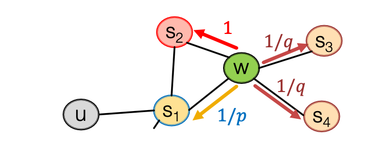
BFS can give a local micro-view of neighborhood, while DFS provides a global macro-view of neighborhood. Here we can define return parameter and in-out parameter and use biased -order random walks to explore network neighborhoods, where models transition probabilities to return back to the previous node and defines the “ratio” of BFS and DFS. Specifically, given a graph below, walker came from edge (, ) and is now at , , and show the probabilities of which node will visit next (here , , and are unnormalized probabilities):
So now are the nodes visited by the biased walk. Let’s put our findings together to state the node2vec algorithm:
- Compute random walk probabilities
- Simulate random walks of length starting from each node
- Optimize the node2vec objective using Stochastic Gradient Descent
TransE
Here we take a look at representation learning on multi-relational graph. Multi-relational graphs are graphs with multiple types of edges, they are incredibly useful in applications like knowledge graphs, where nodes are referred to as entities, edges as relations. For example, there may be one node representing “J.K.Rowling” and another representing “Harry Potter”, and an edge between them with the type “is author of”. In order to create an embedding for this type of graph, we need to capture what the types of edges are, because different edges indicate different relations.
TransE(Bordes, Usunier, Garcia-Duran. NeurIPS 2013.) is a particular algorithm designed to learn node embeddings for multi-relational graphs. We’ll let a multi-relational graph consist of the set of (i.e., nodes), a set of edges , and a set of possible relationships . In TransE, relationships between entities are represented as triplets:
Where is head entity or source-node, is relation and is tail entity or destination-node. Similar to previous methods, entities are embedded in an entity space . The main innovation of TransE is that each relationship is also embedded as a vector .
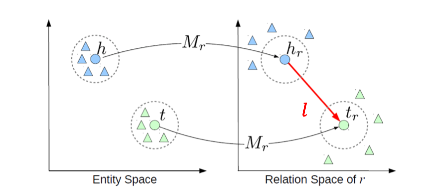
That is, if , TransE tries to ensure that:
Simultaneously, if the edge does not exist, TransE tries to make sure that:
TransE accomplishes this by minimizing the following loss:
Here are “corrupted” triplets, chosen from the set of corruptions of , which are all triplets where either or (but not both) is replaced by a random entity:
Additionally, is a sclar called the , the function is the Euclidean distance, and is the positive part function (defined as max). Finally, in order to ensure the quality of our embeddings, TransE restricts all the entity embeddings to have length , that is, for every :
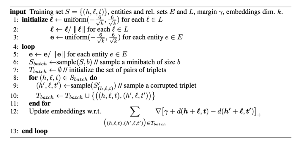
Figure below shows the pseudocode of TransE algorithm:
Graph Embedding
We may also want to embed an entire graph in some applications (e.g., classifying toxic vs. non-toxic molecules, identifying anomalous graphs).
There are several ideas to accomplish graph embedding:
- The simple idea (Duvenaud et al., 2016) is to run a standard graph embedding technique on the (sub)graph , then just sum (or average) the node embeddings in the (sub)graph .
-
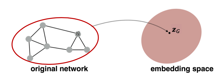
Introducing a “virtual node” to represent the (sub)graph and run a standard graph embedding technique:
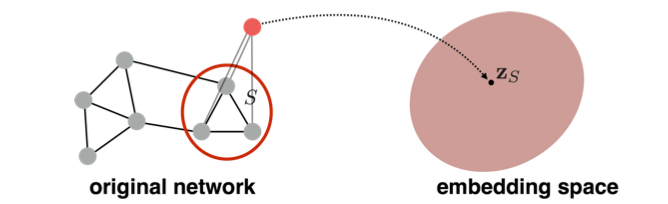 To read more about using the virtual node for subgraph embedding, refer to Li et al., Gated Graph Sequence Neural Networks (2016)
 - We can also use anonymous walk embeddings. In order to learn graph embeddings, we could enumerate all possible anonymous walks of steps and record their counts and represent the graph as a probability distribution over these walks. To read more about anonymous walk embeddings, refer to Ivanov et al., Anonymous Walk Embeddings (2018).