Message Passing and Node Classification

Node Classification

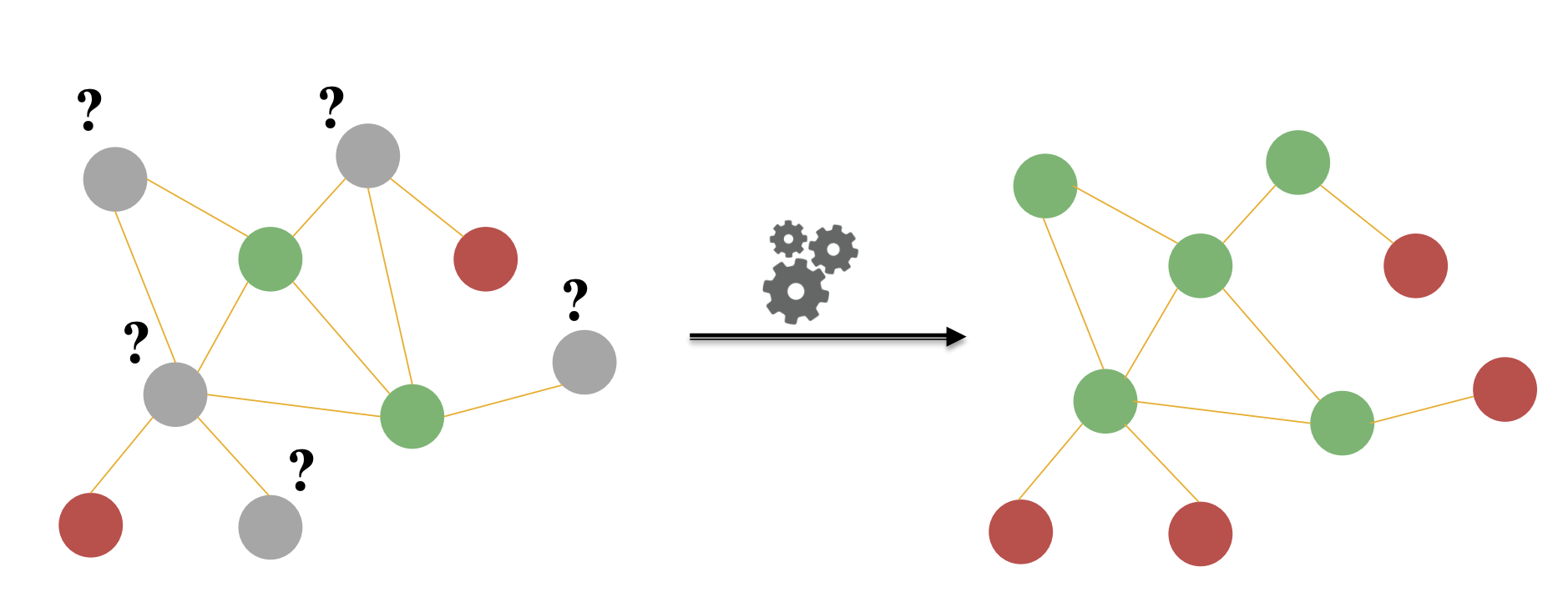
Node Classification is the process of assigning labels to nodes within a graph, given a set of existing node labels. This setting corresponds to a semi-supervised setting. While it would be nice to be able to collect the true label values of every node, oftentimes, in real world settings, it is extremely expensive to collect those labels. Consequently, we rely on random sampling to obtain these labels. Then we use that small sample of labels to develop models that generate trustworthy node label predictions for our graph.

Collective Classification is an umbrella term describing how we assign labels to all nodes in the network together. We then propagate the information from these labels around the network and attempt to come up with stable assignments for each node. We are able to do these tasks because networks have special properties, specifically, correlations between nodes, that we can leverage to build our predictor. Essentially, collective classification relies on the Markov Assumption that the labely $Y_i$ of one node depends on the labels of its neighbors, which can be mathematically written as:

The three main techniques that are used are Relational Classification, Iterative Classification, and Belief Classification, roughly ordered byhow advanced these methods are.

Correlations in a Network

Individual behaviors are correlated in a network environment. These correlations are often the result of three main types of phenomena: Homophily, Influence, and Confounding.

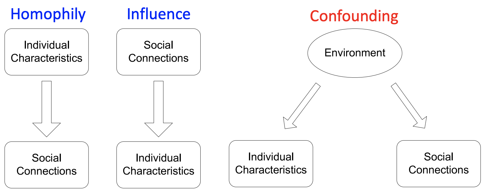
Homophily

“Birds of a feather flock together”

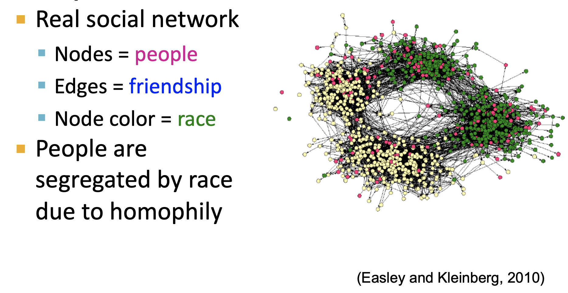
Homophily generally refers to the tendency of individuals to associate and bond with similar others. Similarities, for instance in a social network, can include a variety of attributes, including age, gender, organizational affiliation, taste, and more. For instance, individuals who like the same network may associate more closely together because they meet and interact at concerts or interact in music forums. This phenomena can often be reflected in our friendships, as in the graph below where Easley and Kleinberg (2010) demonstrate the homophily by race in friendships.

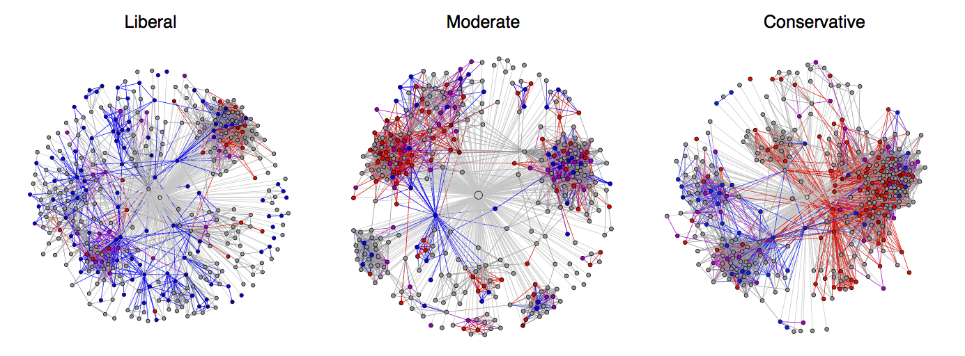
Additionally, in our politics, we can also see this trend. Individuals tend to segregate friendships based on their political views:

Influence

Another example of why networks may demonstrate correlations is Influence. Under these circumstances, the links and edges formed can influence the behavior of the node itself. Think of a social network, where each individual may be influenced by their friends–for instance, a friend may recommend a musical preference which you then become interested in, and you may then pass that preference on to your friends as well.

Confounding

Confounding variables can cause nodes to exhibit similar characteristics. For instance, the environment we are raised in may influence our similarity in multiple dimensions, from the language we speak, to our music tastes, to our political preferences.

Leveraging Network Correlations for Classification of Network Data

“Guilt-by-association”

If a node is connected to another node with a particular label, then that node is more likely to share the same label, as the Markov assumption tells us. For instance, if my friends are all Italian, I am more likely to be Italian myself, based on the network correlations we discussed above. This approach has broad utility across multiple domains, and can be used, for instance, for distinguishing malicious and benign webpages. Malicious webpages tend to link to one another in order to increase visibility, look credible, and rank higher in search engines.

Performing guilt-by-association node classification

Whether or not a particular node X receives a particular label may depend on a variety of factors. In our context, those most commonly include:

• Features of X
• Labels of the objects in X’s neighborhood
• Features of the objects in X’s neighborhood

However, if we were to be using only these features, and not network properties, we would only be training a plain classifier on these featuers. In order for us to perform collective classification, we also need to take into account the network topology. Collective classification requires the 3 components listed below:

• A local classifier to assign initial labels
  • This standard classifier will predict labels based on node attributes/features, without incorporating network information. We can use pretty much any classifier here, even kNNs perform reasonably well.
• A relational classifier is useful because it allows us to capture correlations (e.g. the homophily, influence) between nodes in the network.
  • This classifier predicts the label of one node based on the labels and features of its neighbors.
  • This is the step that incorporates network information.
• Collective inference propagates the correlations through the network. Basically, we do not want to stop at the level of only using our neighbors, but through multiple iterations we want to be able to spread the contribution of other neighbors to each other.
  • This is an iterative series of steps that applies the relational classifer to each node in succession, and iterates until the inconsistency between neighboring node labels is minimized, or until we have reached our maximum iterations and run out of computational resources.
  • Node structure has a profound impact on the final predictions.

There are numerous applications for collective classification, including:

• Document Classification
• Part of speech tagging
• Link prediction
• Optical character recognition
• Image/3D data segmentation
• Entity resolution in sensor networks
• Spam and fraud detection

Example:

For the following graph, we would like to predict labels on the unlabeled, beige nodes as either (+) or (-):

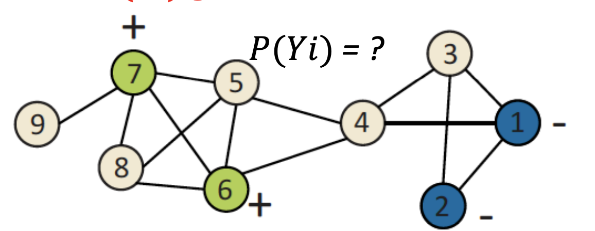
To make those predictions, we will use a Probabilistic Relational Classifier, the basic idea of which is that the class probability of $Y_i$ is a weighted average of the class probabilities of its neighbors. To initialize, we will use the ground-truth labels of our labeled nodes, and for the unlabeled nodes, we will initialize Y uniformly, for instance as $P(Y_{unlabeled}) = 0.5$–or if you have a prior that you trust, you can use that here. After initialization, you may begin to update all nodes, in random order, until convergence conditions or you have reached the maximum number of iterations. Mathematically, each repetition will look like this: $P(Y_i= c) = \frac{1}{\vert N_i\vert}{\sum_{(i,j)\in E} W_{(i,j)}} \sum W_{(i,j)} P(Y_j = c)$

Where $N_i$ is the number of neighbors of i and W is the weighted edge strength from i to j.

We will update the nodes in random order until we reach convergence or our maximum number of iterations. We do not have to update in random order, but it has been shown empirically that it works very well across many cases, so we suggest random ordering. We must remember, however, that our results will be influenced by the order of nodes, especially for smaller graphs (larger graphs are less sensitive to that).

It should be noted, however, that there are 2 additional caveats:

• Convergence is not guaranteed
• Model cannot use node feature information

Iterative Classification

As mentioned in the previous section, relational classifiers do not use node attributes, and so in order to leverage them we use iterative classification which allows you to classify node i based not only on the labels of its neighbors, but on its own attributes in addition. This process consists of the following steps:

• Bootstrap phase
  • create a flat vector $a_i$ for each node i.
  • Train a local classifier, our baseline, $f(a_i)$, (e.g. SVM, kNN) using $a_i$.
  • Aggregate neighbors using count, mode, proportion, mean, exists, etc. We must determine the most sensical way to aggregate our futures.
• Iteration phase
  • Repeat for each node i:
    • Update node vector $a_i$
    • update our label assignment $Y_i$ to $f(a_i)$ which is a hard assignment
  • Iterate until class labels stabilize or max number of iterations is reach

This is very similar to what we did before with the relational classifier, the key difference being that we now use the feature vector and once again, convergence is not guaranteed. You can find a great, real world example of this here .

Message Passing/Belief Propagation

Loopy Belief Propagation

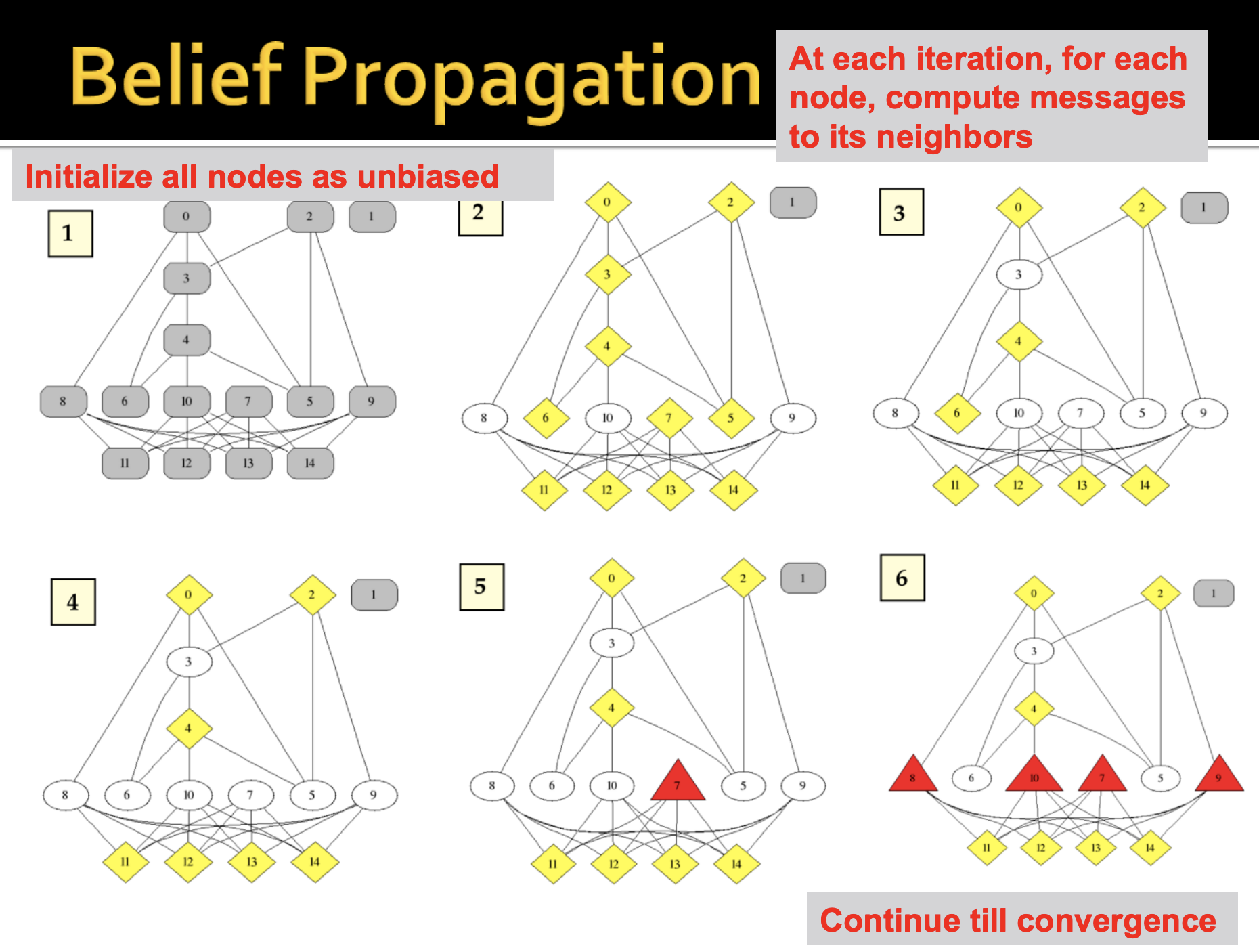
Belief propagation is a dynamic programming technique that answers conditional probabiliy queries in a graphical model. It’s an iterative process in which every neighbor variables talk to each other, by passing messages.

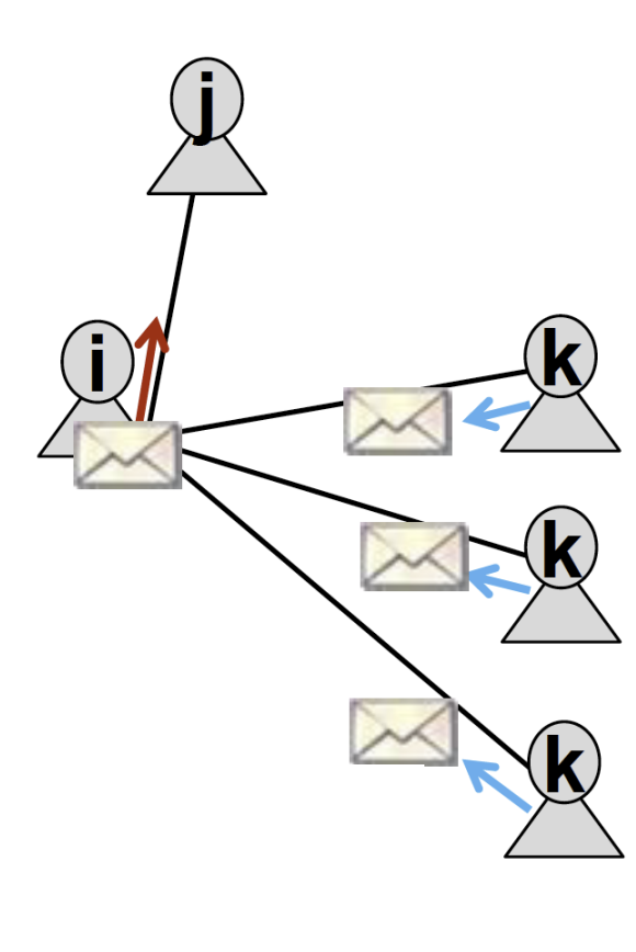
For instance, I (variable $x_1$) might pass a message to you (variable $x_2$) stating that you belong in these states with these different likelihoods. The state of the node in question doesn’t depend on the belief of the node itself, but on the belief of all the nodes surrounding it.

What message node i ends up sending to node j ultimately depends on its neighbors, k. Each neighbor k will pass a message to i regarding its belief of the state of i, and then i will communicate to j.

When performing belief propagation, we will need the following notation:

Notation:

• Label-Label potential matrix $\psi$ represents the dependency between a node and its neighbor. $\psi (Y_i, Y_j)$ is simply equal to the probability of a node j being in state $Y_j$ given that its neighbor i is in state $Y_i$. We have been seing this with the other methods, we just formalize it here. It basically captures what is the correlation between node i and j.
• Prior belief $\phi$ or $\phi (Y_i)$ represents the probability of node i being in state $Y_i$. This is capturing the node features.
• m$_{i\to j}(Y_j)$ is the message from i to j, which represents i’s estimate of j being in state $Y_j$.
• $\mathcal{L}$ represents the set of all states.

Once we have all notation, we can compile this all together to give us the message that i will send to j for state $Y_j$.

$m_i\to_j(Y_j) = \alpha \sum \psi (Y_i, Y_j) \phi_i(Y_i)\Pi_{k \in \mathcal{N}\backslash j} m_{k\to i}$ $\forall \mathcal{L}$

This equation summarizes our task: to calculate the message from i to j, we will sum over all of our states the label-label potential multiplied by our prior, multiplied by the product of all the messages sent by neighbors from the previous rounds. To initialize, we set all of our messages equal to 1. Then, we calculate our message from i to j, using the formula described above. We will repeat this for each node until we reach convergence, and then we can calculate our final assignment, i’s belief of being in state $Y_i$, or $b_i(Y_i)$.

Belief propagation has many advantages. It’s easy to program and easy to parallelize. Additionally, it’s very general and can apply to any graphical model with any form of potentials (higher order pairwise). However, similar to the other techiques, convergence is once again, not guaranteed. This is particularly an issue when their are many closed loops. It should be noted that we may also learn our priors.

A good example of Belief Propagation in action is detection of online auction fraud.