Graph Neural Networks

In the previous section, we have learned how to represent a graph using “shallow encoders”. Those techniques give us powerful expressions of a graph in a vector space, but there are limitations as well. In this section, we will explore three different approaches using graph neural networks to overcome the limitations.

Limitations of “Shallow Encoders”

Shallow Encoders do not scale, as each node has a unique embedding.
Shallow Encoders are inherently transductive. It can only generate embeddings for a single fixed graph.
Node Features are not taken into consideration.
Shallow Encoders cannot be generalized to train with different loss functions.

Fortunately, graph neural networks can solve the above limitations.

Graph Convolutional Networks (GCN)

Traditionally, neural networks are designed for fixed-sized graphs. For example, we could consider an image as a grid graph or a piece of text as a line graph. However, most of the graphs in the real world have an arbitrary size and complex topological structure. Therefore, we need to define the computational graph of GCN differently.

Setup

Given a graph $G = (V, A, X)$ such that:

$V$ is the vertex set
$A$ is the adjacency matrix
$X\in \mathbb{R}^{m\times\rvert V \rvert}$ is the node feature matrix

Computational Graph and Generalized Convolution

aggregate_neighbors

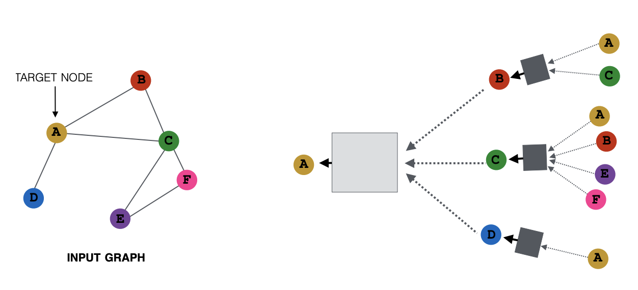
Let the example graph (referring to the above figure on the left) be our $G$ . Our goal is to define a computational graph of GCN on $G$ . The computational graph should keep the structure of $G$ and incorporate the nodes’ neighboring features at the same time. For example, the embedding vector of node $A$ should consist of its neighbor $\{B, C, D\}$ , and not depend on the ordering of $\{B, C, D\}$ . One way to do this is to simply take the average of the features of $\{B, C, D\}$ . In general, the aggregation function (referring to the boxes in the above figure on the right) needs to be order invariant (max, average, etc.). The computational graph on $G$ with two layers will look like the following:

computation_graph

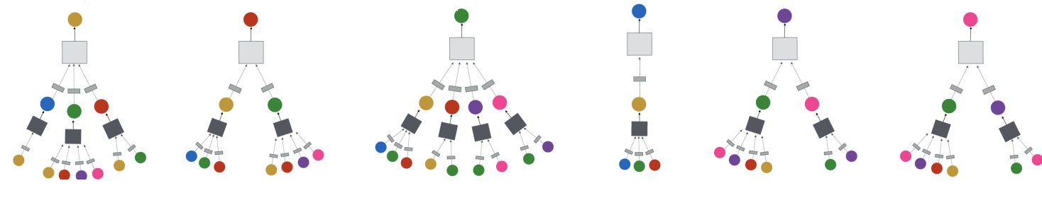
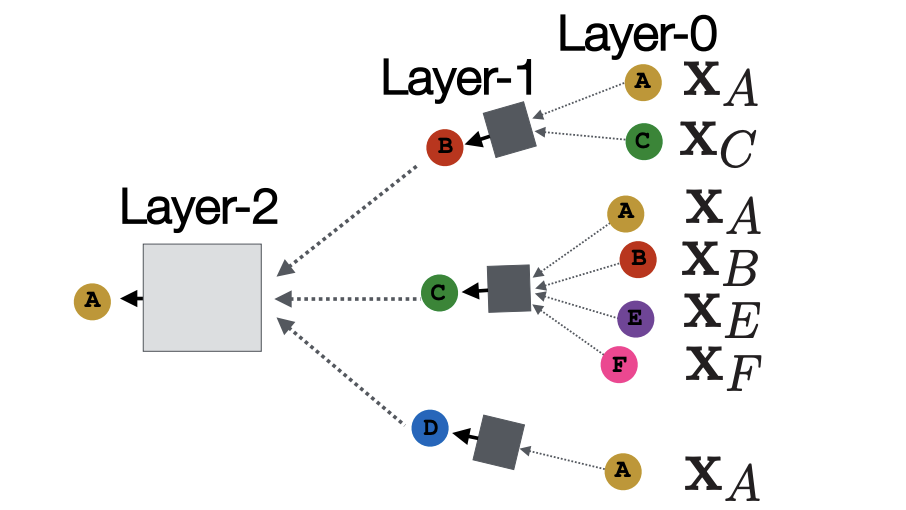
Here, each node defines a computational graph based on its neighbors. In particular, the computational graph for node $A$ can be viewed as the following (Layer-0 is the input layer with node feature $X_i$ ):

computation_graph_for_a

Deep Encoders

With the above idea, here is the mathematical expression at each layer for node $v$ using the average aggregation function:

At 0th layer: $h^0_v = x_v$ . This is the node feature.
At kth layer: $h_v^{k} = \sigma(W_k\sum_{u\in N(v)}\frac{h_u^{k-1}}{\rvert N(v)\rvert} + B_kh_v^{k-1}), \forall k \in \{1, .., K\}$ .

$h_v^{k-1}$ is the embedding of node $v$ from the previous layer. $\rvert N(v) \rvert$ is the number of the neighbors of node $v$ . The purpose of $\sum_{u\in N(v)}\frac{h_u^{k-1}}{\rvert N(v) \rvert}$ is to aggregate neighboring features of $v$ from the previous layer. $\sigma$ is the activation function (e.g. ReLU) to introduce non-linearity. $W_k$ and $B_k$ are the trainable parameters.

Output layer: $z_v = h_v^{K}$ . This is the final embedding after $K$ layers.

Equivalently, the above computation can be written in a matrix multiplication form for the entire graph:

$H^{l+1} = \sigma(H^{l}W_0^{l} + \tilde{A}H^{l}W_1^{l})$ such that $\tilde{A}=D^{-\frac{1}{2}}AD^{-\frac{1}{2}}$ .

Training the Model

We can feed these embeddings into any loss function and run stochastic gradient descent to train the parameters. For example, for a binary classification task, we can define the loss function as:

$L = \sum_{v\in V} y_v \log(\sigma(z_v^T\theta)) + (1-y_v)\log(1-\sigma(z_v^T\theta))$

$y_v \in \{0, 1\}$ is the node class label. $z_v$ is the encoder output. $\theta$ is the classification weight. $\sigma$ can be the sigmoid function. $\sigma(z_v^T\theta)$ represents the predicted probability of node $v$ . Therefore, the first half of the equation would contribute to the loss function, if the label is positive ( $y_v=1$ ). Otherwise, the second half of the equation would contribute to the loss function.

We can also train the model in an unsupervised manner by using: random walk, graph factorization, node proximity, etc.

Inductive Capability

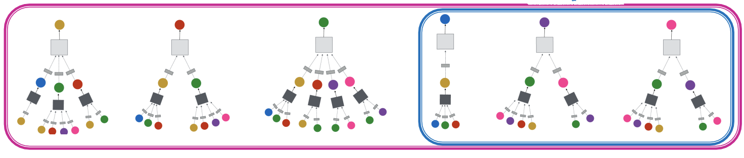
GCN can be generalized to unseen nodes in a graph. For example, if a model is trained using nodes $A, B, C$ , the newly added nodes $D, E, F$ can also be evaluated since the parameters are shared across all nodes. apply_to_new_nodes

GraphSAGE

So far we have explored a simple neighborhood aggregation method, but we can also generalize the aggregation method in the following form:

$h_v^{K} = \sigma([W_k AGG(\{h_u^{k-1}, \forall u \in N(v)\}), B_kh_v^{k-1}])$

For node $v$ , we can apply different aggregation methods ( $AGG$ ) to its neighbors and concatenate the features with $v$ itself.

Here are some commonly used aggregation functions:

Mean: Take a weighted average of its neighbors.

$AGG = \sum_{u\in N(v)} \frac{h_u^{k-1}}{\rvert N(v) \rvert}$

Pooling: Transform neighbor vectors and apply symmetric vector function ( $\gamma$ can be element-wise mean or max).

$AGG = \gamma(\{ Qh_u^{k-1}, \forall u\in N(v)\})$

LSTM: Apply LSTM to reshuffled neighbors.

$AGG = LSTM(\{ h_u^{k-1}, \forall u\in \pi(N(v)\}))$

Graph Attention Networks

What if some neighboring nodes carry more important information than the others? In this case, we would want to assign different weights to different neighboring nodes by using the attention technique.

Let $\alpha_{vu}$ be the weighting factor (importance) of node $u$ ’s message to node $v$ . From the average aggregation above, we have defined $\alpha=\frac{1}{\rvert N(v) \rvert}$ . However, we can also explicitly define $\alpha$ based on the structural property of a graph.

Attention Mechanism

Let $\alpha_{uv}$ be computed as the byproduct of an attention mechanism $a$ , which computes the attention coefficients $e_{vu}$ across pairs of nodes $u, v$ based on their messages:

$e_{vu} = a(W_kh_u^{k-1}, W_kh_v^{k-1})$

$e_{vu}$ indicates the importance of node $u$ ’s message to node $v$ . Then, we normalize the coefficients using softmax to compare importance across different neighbors:

$\alpha_{vu} = \frac{\exp(e_{vu})}{\sum_{k\in N(v)}\exp(e_{vk})}$

Therefore, we have:

$h_{v}^k = \sigma(\sum_{u\in N(v)}\alpha_{vu}W_kh^{k-1}_u)$

This approach is agnostic to the choice of $a$ and the parameters of $a$ can be trained jointly with $W_k$ .