Generative Models for Graphs

In the Node Representation learning section, we saw several methods to “encode” a graph in the embedding space while preserving the nodes’ similarity and network structure. In this section, we will study how to express probabilistic dependencies among a graph’s nodes and edges and generate new realistic graphs by drawing samples from the learned distribution. This ability to capture the distribution of a particular family of graphs has many applications. For instance, sampling a graph from the generative model trained on a particular family of graphs can lead to the discovery of new configurations that share the same global properties as is, for example, required in drug discovery. Another application of these methods is the ability to simulate “What-If” scenarios in a real-world graph to gather insights about the network properties and attributes.

Challenges

1. For a graph of $n$ nodes, there are $O(n^2)$ possible edges which results in a quadratic explosion while predicting edges in the graph.
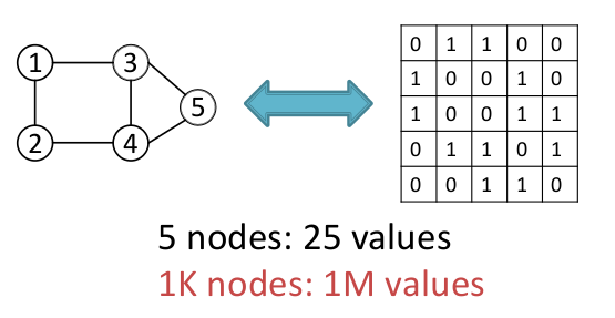
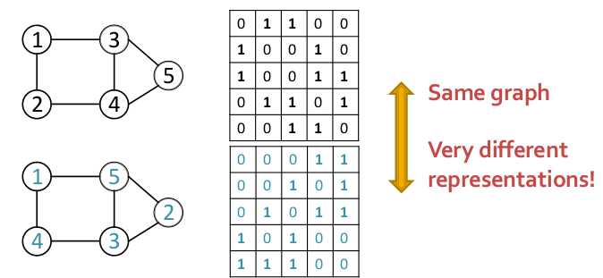
2. $n$-node graph can be represented in $n!$ ways which makes it very hard to optimize objective functions as 2 very different adjacency matrix representations of graphs can result in the same graph structure.
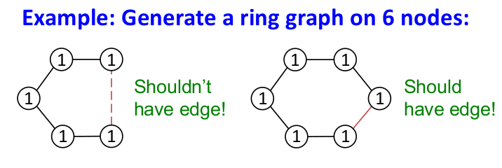
3. Edge formation can have long-range dependencies (e.g. to generate a graph having a 6-node cycle, need to remember the structure so far)

Terminology

1. $p_{data}(G)$: Probability distribution from which a given graph is sampled.
2. $p_{model}(G;\theta)$: The distribution, parametrized by $\theta$, learned by the model to approximate $p_{data}(G)$

Goal: Our goal is 2-fold.

1. Make sure that $p_{model}(G;\theta)$ is very close to $p_{data}(G)$ (Key Idea: Maximum Likelihood)
2. Furthermore, we also need to make sure that we can efficiently sample graphs from $p_{model}(G;\theta)$ (Key Idea: Sample from noise distribution and transform the sampled noise via a complex function to generate the graph)

GraphRNN

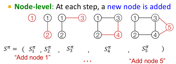
The idea is to treat the task of graph generation as a sequence generation task. We want to model the probability distribution over the next “action” given the previous state of actions. In language modeling, the action is the word we are trying to predict. In the case of graph generation, the action is to add a node/edge. As discussed above, a graph can have multiple sequences associated with it($O(n!)$) but we can map out a unique sequence by ordering the nodes of the graph.

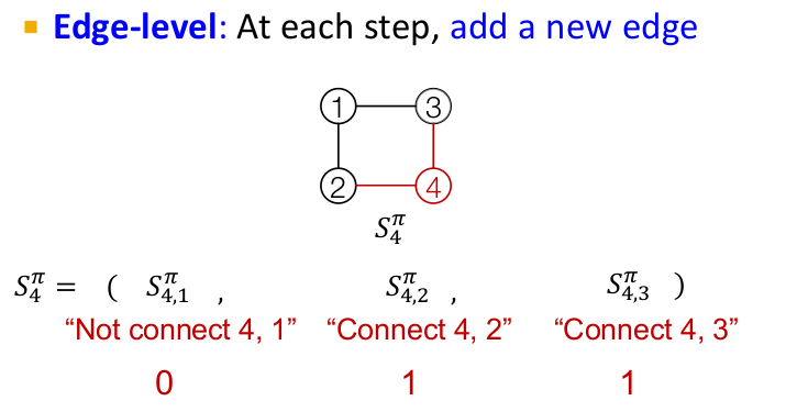
Once the node sequence is fixed, we can map the sequence in which the corresponding edges need to be added to the graph. Thus, the task of graph generation can be equivalently transformed to a sequence generation problem at two levels, first at the node level and then at the edge level. Since RNN are well known for their sequence generation capabilities, we will study how they can be utilized for this task.

GraphRNN has a node-level RNN and an edge-level RNN. The two RNNs are related as follows:

1. Node-level RNN generates the initial state for edge-level RNN
2. Edge-level RNN generates edges for the new node, then updates node-level RNN state using generated results

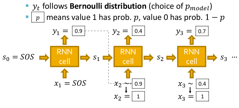
This results in the following architecture. Notice that the model is auto-regressive as the output of the present RNN cell is fed as input to the next RNN cell. Also to make the model more expressive and model a probability distribution, the input for a cell is sampled from its previous cell’s output assuming a Bernoulli distribution. Hence at the inference time, we just pass the special “Start of Sequence(SOS)” token to start the process of sequence generation which happens until an “End of Sequence(EOS)” token is generated.

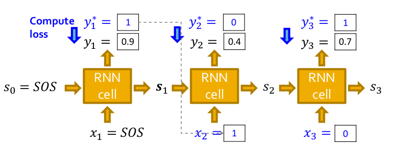
Now we have seen how to generate a graph assuming we have a trained model. But how do we train it? We use the teacher-forcing technique to train the model and replace the input and output by the actual sequence as shown below and use the standard binary cross-entropy loss as the optimization objective which is backpropagated through time(BPTT) to update the model parameters.

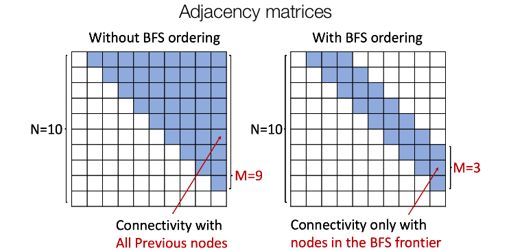
Now we can generate graphs by sampling from a distribution learned by our model. But, the major challenge still remains. Since any node can connect to any prior node, we need to generate half of the adjacency matrix which can turn out to be extremely inefficient due to the problem of quadratic explosion. To tackle this, we generate the node sequence in a BFS manner. This reduces the possible node orderings from $O(n!)$ to a comparatively small distinct BFS orderings and also reduces the number of steps for the edge generation (since now the model doesn’t need to check for all the nodes for connectivity as the node can only connect to its predecessors in the BFS tree) as shown in the following figure.

Further reading: GraphRNN: Generating Realistic Graphs with Deep Auto-regressive Models (ICML 2018)